One of the primary bottlenecks to all-optical data centre networks is the lack of a packet-timescale switch. This project saw the application of AI techniques to switch semiconductor optical amplifiers in just half a nanosecond. AI beat the previous world-record by an order of magnitude and, for the first time, offered the potential to be scaled to thousands of switches in a real data centre.
The Control Problem (Cars)
If you have ever driven a car with cruise control, you will have experienced the solution to a problem that is similar to the challenge of switching light on ultra-fast timescales.
As a car in cruise control approaches a hill, the speed of the car will decrease when it begins to climb the hill, since the throttle is constant. If the driver wants to maintain the speed they had on flat ground, they will have to control the throttle/brakes.
The driver could put the throttle at full power, quickly restoring the speed of the car, but also likely making the car accelerate too much. In this sense, the driver has overshot their target speed, since the car will accelerate beyond the desired speed. The driver will then have to use the brakes, which if not done very precisely may mean the car slows down too much, and the throttle has to be applied again, and so on...
Alternatively, the driver could slowly increase the throttle, paying attention to the car’s speed and keeping the throttle constant when the speed matches the target. While the car achieves the desired speed, it takes a while to do so.
The throttle power at each point in time can be plotted to show the signal that 'controls' the car's speed. This signal can then be related to the performance of the car (I.e. its speed at each corresponding point in time). Therefore, the problem of ensuring the car maintains constant speed can be solved in terms of finding the optimal throttle signal that produces the best (most constant) car performance signal. The response of 'control systems' like these are typically characterised by 3 key metrics:
Rise time: The amount of time taken for the response signal to initially ascend from its lower to its higher value within some margin (e.g. 10% - 90% of final value, referred to as the ‘steady state’)
Settling time: The amount of time taken for the response signal to be and remain within a certain margin of its final value (typically +/- 5% of the final value)
Overshoot: The amount by which the signal exceeds the steady state value on its initial rise, given as a percentage of the excess relative to the desired signal value.
Optical Switching in Data Centres: Semiconductor Optical Amplifiers (SOAs)
Information can be encoded in many different media. It has long been known that light waves/photons are the best medium for encoding and communicating information. Light is usually communicated by passing it through a glass fibre. But how do we control where the light goes such that the information ends up at, and only at, the desired destination? The answer is with a switch.
Optical networks already dominate modern communication networks such as the large fibre optic cables on the seabed that allow internet data to flow across the Atlantic between the USA and Europe. Although we refer to these networks as optical, in fact they are partially still electronic. This is because at each mid-way point/node in the network, the optical signal must be converted to an electronic signal as the information is switched towards its destination. In long-haul communication, the data flows (packets of data being sent) are long and so don’t have to be routed often, meaning network switches do not have to be able to reconfigure/switch the light at high speeds. In data centres, on the other hand, data flows are typically on the order of 10 ns, so slow switches will mean that more time is spent waiting for the network to reconfigure between flows than is spent allowing the flows to be transported. The time it takes to reconfigure the network relative to the length of the data packet is referred to as the switching overhead and leads to unacceptable latencies in data centres. To solve this, fast switches capable of all-optical switching (i.e. no overhead needed for optical-electrical-optical signal conversion) are needed.
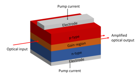
The most promising technology for ultra-fast all-optical switching is the 'semiconductor optical amplifier' (SOA). SOAs are relatively simple ‘amplification’ devices, and work in the same way as common everyday lasers; they use the quantum mechanical effects of spontaneous emission, stimulated emission, and stimulated absorption to amplify light and to operate as optical switches and wavelength converters. They typically have the following structure:
Structure of a typical semiconductor optical amplifier (SOA) device.
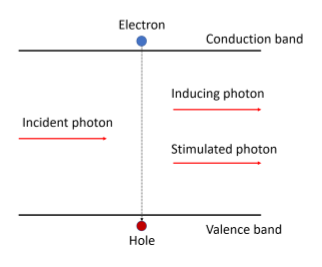
To amplify light, the ‘gain region’ (the region light comes into and out of) is sandwiched between an ‘n-type’ material (a material with many electrons in the conduction band) and a ‘p-type’ material (a material with many holes (absent electrons) in the valence band). A driving pump current is applied via metal electrodes to the n-type and p-type materials to supply electrons and holes respectively. The excess holes and electrons pass into the gain region’s valence and conduction bands respectively, forming hole-electron pairs (‘excitons’). An optical input signal is passed into the SOA gain region, stimulating electrons to recombine with holes by stimulated emission. This process causes a photon of energy/wavelength equal to the incumbent photon’s wavelength to be released, thereby creating an amplified optical output signal.
Diagram of the stimulated emission process.
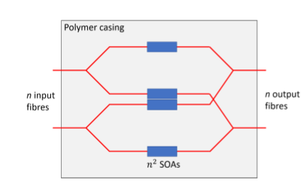
To route light along a specific path, one SOA can be placed on each possible path. The SOA on the desired path has an electrical current drive signal applied to it to turn it ‘on’ (i.e. to make it amplify the light), and the other SOAs remain ‘off’ to make them absorb the light and prevent information reaching undesired destinations. This constitutes a simple SOA-based optical switch:
Diagram of how SOAs can be used in an SOA-based optical switch system.
Since SOAs are an all-optical technology, they do not need to undergo optical-electrical-optical conversion like conventional electronic switches, which is a major bottleneck for switching speeds. In theory, the switching speed of an SOA switch is limited by the carrier recombination lifetime (how long it takes a hole and an electron to recombined), which is on the order of a hundred picoseconds. As such, SOA switches open the possibility of ultra-fast sub-nanosecond switching, thereby reducing network latency and enabling all-optical data centre networks.
The Control Problem (SOAs)
Much like the control problem with cruise control systems in cars, applying a simple electrical signal to turn ‘on’ an SOA results in overshoot, rise time and settling time issues.
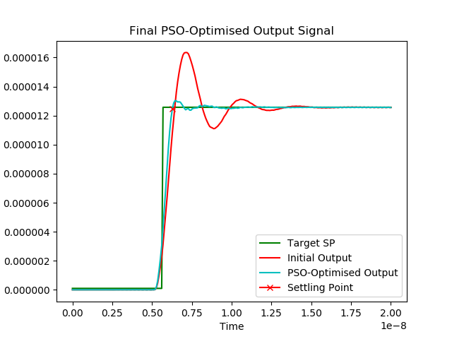
The switch speed (off-on time) of an SOA is typically characterised in terms of rise time. However, due to various interactions within the SOA, a fast rise time typically leads to ‘ringing’ (oscillations around the steady state value) as described in relation to cars using cruise control. This ringing is not accounted for in the rise time metric. The rise time typically occurs on the order of hundreds of picoseconds, but the ringing can persist for the order of nanoseconds (see red curve in the figure below).
If SOAs are applied to signals on which data is to be encoded, significant ringing can mean that the encoded symbols cannot be easily read and/or distinguished, since the value of the SOA output is inconsistent. This introduces noise/errors into the data communication and means that the SOA can not realistically be used.
Characterising SOA switching speed in terms of settling time is therefore more useful. If the SOA has settled, then it’s output power level is consistent within a defined margin, meaning that data can be reliably transferred with that signal. In a data centre, data packets are quite short, typically lasting for about ~20 nanoseconds. The network needs to be able to re-configure in some way for each packet. If this takes significantly longer than the duration of the packet, then the network spends more time re-configuring then it does transmitting, meaning it is incredibly inefficient. This therefore motivates the goal of finding a driving signal that can reduce the SOA switching speed (as given by the settling time, not rise time) as much as possible. This is equivalent to finding an SOA driving signal that produces an SOA output close to that of a perfect step signal.
Some key considerations guided our work in finding an appropriate way of optimising SOAs:
In the context of large DC networks, the method must be easily applicable to 100,000s or more SOA (i.e. the method cannot require meticulous hand-tuning upon each application instance)
Results must be consistent across different types of SOAs
Previous attempts at ultra-fast SOA switching had to hand-build a drive signal based on assumptions about the SOAs material structure, and its mounting electronics. However, these methods are very limited (any arbitrary signal cannot be produced, since the process is restricted by assumptions made about the system) and non-transferrable (they are designed for a specific SOA with no demonstration of generality).
To solve this problem, we used artificial intelligence (AI) techniques that can find the optimum electrical drive signal needed for the SOAs in a fully automated fashion. Unlike other methods, our AI algorithms required no prior knowledge of the SOA, and could therefore be generalised to any SOA-based optical switch. The AI techniques not only achieved a ~10x improvement in the settling time (the effective switch speed), achieving 0.5 nanosecond settling times in experiment, but due to their automated nature, can also easily be scaled and applied to millions of unseen SOAs in a real data centre.
Optical responses of an SOA to an initial step signal (the 'initial output', red) and a PSO-optimised signal (the 'PSO-optimised output, cyan). The target 'perfect step' set point (SP) has also been plotted (green). The PSO signal achieves much faster settling time than the step signal, and therefore has a much quick switching speed.
How the AI Technique Works: Particle Swarm Optimisation (PSO)
Three AI techniques were compared for optimising the SOA drive signal; particle swarm optimisation (PSO), ant colony optimisation (ACO), and a genetic algorithm (GA). Of these, the technique with the best performance and generality was PSO (optimised optical response shown in previous diagram).
PSO is a population-based artificial intelligence metaheuristic. First proposed in 1995 by [1], it combines swarm theory by observing natural phenomena such as bird flocks and fish schoools with evolutionary programming. In this project, PSO was adapted to be applicable to any SOA drive signal optimisation scenario.
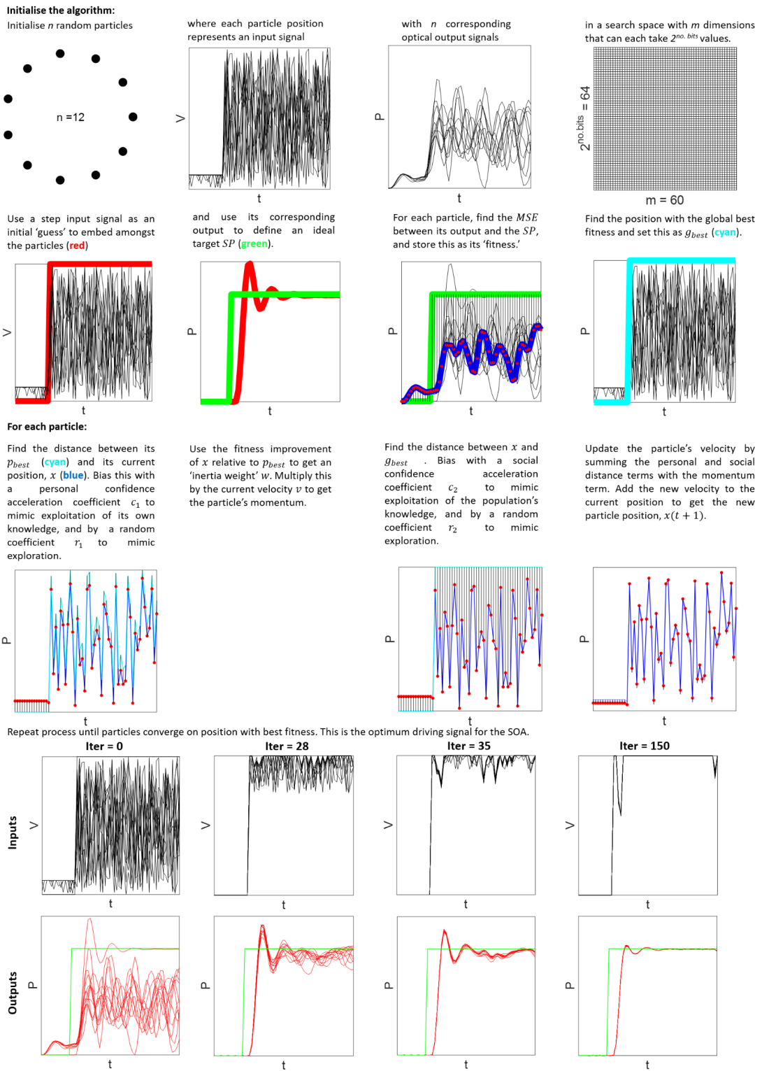
A population of $n$ particles were initialised at random positions in a hyperdimensional search space with $m$ dimensions describing each position. In the case of SOA switching, $x_j (t)$ denoted the position (amplitudes taken) $x$ of particle (driving signal) $j$ at time (discrete point in the signal period) $t$. The particle was flown through the search space by updating its position at each sequential iteration/generation by adding a velocity $v_j (t)$ to its position: $$x_j(t+1) = x_j (t) + v_j (t+1)$$ The velocity vector was what drove the optimisation process. It contained the personal knowledge of the particle (the 'cognitive component', which was proportional to the distance between $x_j (t)$ and its historic personal best position $p_{best_j}$) as well as the socially exchanged information of the particle's neighbours (the 'social component', which was proportional to the distance between $x_j(t)$ and the whole swarm's historic global best position $g_{best}$). The velocity was updated according to: $$ v_{jg}(t+1) = w_j \cdot v_{jg}(t) + c_{1j} \cdot r_{1j}(t) \cdot \left[ p_{best_{jg}}(t) - x_{jg}(t) \right] + c_{2j} \cdot r_{2j}(t) \cdot \left[g_{best_{g}} - x_{jg} \right] $$ Where $v_{jg}(t)$ was the velocity of particle $j$ in dimension (point in the signal) $g~=~\{1, 2, ..., m\}$ at time $t$, $c_{1j}$ and $c_{2j}$ were the personal and social 'confidence acceleration constants' of particle $j$ used to scale the contributions of the cognitive and social components respectively, $r_{1j}$ and $r_{2j}$ were random values in the range [0, 1] sampled from a uniform distribution in order to introduce a stochastic element to PSO resembling 'exploration', and $w_j$ was the 'inertia weight' or 'momentum' of particle $j$ used to control the exploration and exploitation inclinations of the particle. A higher $c_1$ encouraged the particle to be more confident in itself and explore more positions but possibly take longer to converge on the optimum $g_{best}$, whereas a higher $c_2$ encouraged the particle to trust the social knowledge of its neighbours and converge faster on $g_{best}$ but be less inclined to explore new positions. These coefficient values were critical since they balanced exploration and exploitation and controlled convergence time. So long as they satisfied the below equation, PSO was guaranteed to converge on some driving signal state. $$ 0 \leq \frac{1}{2} \left( c_1 + c_2 \right) - 1 < w < 1 $$ To avoid being either too exploitative or too exploratory, $w$, $c_1$ and $c_2$ were dynamically updated according to the following: $$ w_j(t+1) = w(0) + \left[ \left( w(n_t) - w(0) \right) \cdot \left( \frac{e^{m_j(t)} -1} {e^{m_j(t)} + 1} \right) \right] $$ $$ m_j(t) = \frac{p_{best_j}(t) - x_j(t)}{p_{best_j}(t) + x_j(t)} $$ $$ c_{1,2}(t) = \frac{c_{min} + c_{max}}{2} + \frac{c_{max} - c_{min}}{2} + \frac{e^{-m_j(t)}-1}{e^{-m_j(t)} + 1} $$ Where $w(0)$ was the initial inertia weight constant ($0~\leq~w(0)~<~1$), $w(n_t)$ was the final inertia weight constant ($w(0) > w(n_t)$), $m_j(t)$ was the relative fitness improvement of particle $j$ at time $t$, and $c_{max}$ and $c_{min}$ were the maximum and minimum values for the acceleration constants.
To evaluate a given particle position/driving signal, a fitness function $f$ was defined as being the mean squared error (MSE) between the actual SOA output and an ideal SOA step output with 0 rise time, 0 settling time and 0 overshoot. The closer a driving signal's corresponding output 'process variable' (PV) was to achieving this ideal 'set point' (SP), the lower its fitness value. This was therefore a minimisation problem, whereby $p_{best}$ and $g_{best}$ could be updated according to the below equations respectively. $$ f = \frac{1}{m} \sum_{g=0}^{m} \left( PV - SP \right)^2 $$ $$ p_{best_j}(t+1) = \begin{cases} p_{best_j}(t), & \text{if $f(x_j(t+1)) \geq f(p_{best_j}(t))$} \\ x_j(t+1), & \text{otherwise} \end{cases} $$ $$ g_{best}(t+1) = \begin{cases} g_{best}(t), & \text{if $f(x_j(t+1)) \geq f(g_{best}(t))$} \\ x_j(t+1), & \text{otherwise} \end{cases} $$
This PSO process could be repeated until the particles converged on a position with the best fitness, which corresponded to the optimum driving signal for the SOA. Below is a visual representation of the above applied to a simplified scenario.
Visualisation of the PSO algorithm optimising the drive signal of an SOA.